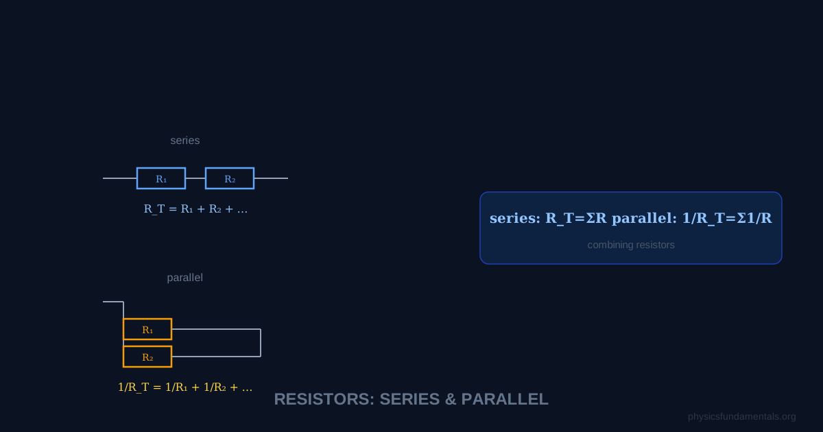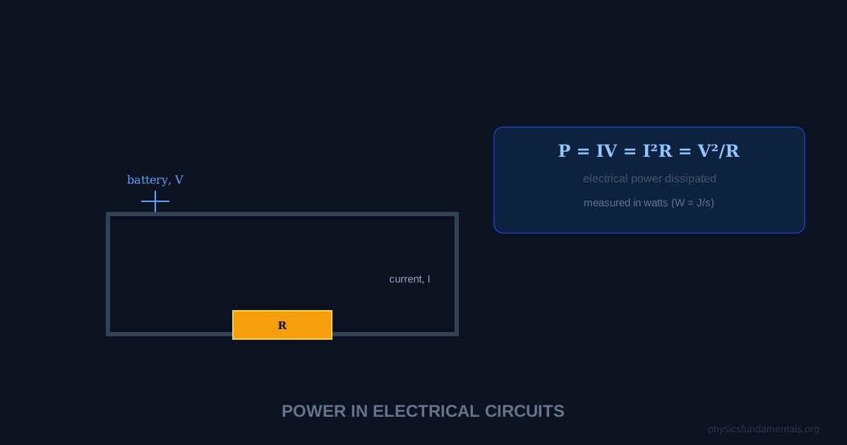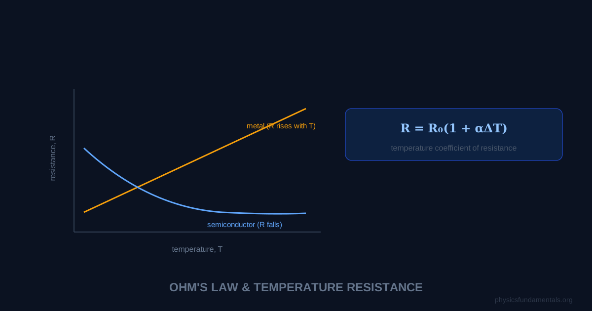
Kirchhoff's Laws: Solving Multi-Loop Circuits Step by Step

Kirchhoff's laws provide the systematic method for analysing any circuit, no matter how complex. Kirchhoff's Current Law (KCL): the sum of currents entering any junction equals the sum leaving it. Kirchhoff's Voltage Law (KVL): the sum of all voltage changes around any closed loop is zero. Applied together with a methodical procedure — assign currents, write KCL equations at junctions, write KVL equations around loops, solve simultaneously — they can solve any resistive circuit. This article extends the introduction in our Kirchhoff's Laws fundamentals article to multi-loop circuits.

Multi-loop circuits — those with more than one independent loop — cannot be reduced to simple series and parallel combinations. They require the full Kirchhoff's law treatment. The approach is systematic and algorithmic: follow the steps in order and the equations write themselves.

The Systematic Procedure

1. Label all junctions (points where three or more wires meet) with letters (A, B, C...).
2. Assign a current to each branch (each wire between two junctions). Label them I₁, I₂, I₃... Choose a direction for each — if you guess wrong, the answer will just be negative, which tells you the actual current flows opposite to your assumed direction.
3. Apply KCL at junctions: for each independent junction, write ΣI_in = ΣI_out. For a circuit with n junctions, write n−1 independent KCL equations (the nth is not independent).
4. Apply KVL around loops: choose independent loops and traverse them in any direction. For each element: +EMF when crossing battery − to +; −IR when crossing resistor in the direction of assumed current; +IR against the assumed current direction. Set each loop sum to zero.
5. Solve the simultaneous equations for all unknown currents.
6. Check: verify that the solutions satisfy all KCL and KVL equations and that total power delivered by sources equals total power dissipated in resistors.

Sign Conventions for KVL

Traversing a loop, add voltage changes as follows:

Element crossed	Traversal direction	Voltage change
Battery (EMF ε)	− terminal to + terminal	+ε (gain)
Battery (EMF ε)	+ terminal to − terminal	−ε (drop)
Resistor R, current I	In direction of assumed current I	−IR (drop)
Resistor R, current I	Against direction of assumed current I	+IR (gain)

3 Fully Worked Examples

Example 1 — Two batteries, three resistors (T-circuit)

Circuit: Battery ε₁ = 12 V (internal resistance r₁ = 1 Ω) in the left branch, battery ε₂ = 6 V (r₂ = 1 Ω) in the right branch, both connected to a common 4 Ω resistor R₃ in the middle branch. All three branches connect between nodes A (top) and B (bottom).

Step 1 — Assign currents: I₁ flows down from ε₁ through r₁; I₂ flows down from ε₂ through r₂; I₃ flows down through R₃.

Step 2 — KCL at node A: I₁ + I₂ = I₃ (currents from left and right branches combine into middle)

Step 3 — KVL around left loop (clockwise: A → through ε₁ → through r₁ → B → through R₃ → back to A):
+ε₁ − I₁r₁ − I₃R₃ = 0
12 − I₁(1) − (I₁ + I₂)(4) = 0
12 = 5I₁ + 4I₂ ... (equation 1)

Step 4 — KVL around right loop (clockwise: A → through ε₂ → through r₂ → B → through R₃ → back to A):
+ε₂ − I₂r₂ − I₃R₃ = 0
6 − I₂(1) − (I₁ + I₂)(4) = 0
6 = 4I₁ + 5I₂ ... (equation 2)

Step 5 — Solve simultaneously:
From (1): 12 = 5I₁ + 4I₂
From (2): 6 = 4I₁ + 5I₂
Multiply (1) by 5 and (2) by 4: 60 = 25I₁ + 20I₂ and 24 = 16I₁ + 20I₂
Subtract: 36 = 9I₁ → I₁ = 4 A
From (2): 6 = 16 + 5I₂ → I₂ = −2 A (current actually flows up in right branch)
I₃ = I₁ + I₂ = 4 − 2 = 2 A

Check power:
Power from ε₁ = ε₁I₁ = 12 × 4 = 48 W
Power from ε₂ = ε₂|I₂| = 6 × 2 = 12 W (ε₂ is being charged, not supplying)
Actually: ε₂ absorbs power = 6 × 2 = 12 W
Dissipated: I₁²r₁ + I₂²r₂ + I₃²R₃ = 16×1 + 4×1 + 4×4 = 16+4+16 = 36 W
Net supply = 48 − 12 = 36 W ✓

Example 2 — Wheatstone bridge (unbalanced)

Circuit: 10 V battery, with resistors: R₁ = 2 Ω (top-left), R₂ = 4 Ω (top-right), R₃ = 3 Ω (bottom-left), R₄ = 6 Ω (bottom-right), and R₅ = 5 Ω (bridge between middle nodes). Find the current through R₅.

Assign currents: I₁ through R₁, I₂ through R₂, I₃ through R₃, I₄ through R₄, I₅ through R₅. Let nodes be: A (battery +), C (top middle), D (bottom middle), B (battery −).

KCL:
At C: I₁ = I₂ + I₅
At D: I₃ + I₅ = I₄
At A: I = I₁ + I₃ (total current from battery)

KVL — Loop 1 (A→C→B via R₁, R₂): 10 − 2I₁ − 4I₂ = 0
KVL — Loop 2 (A→D→B via R₃, R₄): 10 − 3I₃ − 6I₄ = 0
KVL — Loop 3 (C→D via R₅, up through R₃ to A to C via R₁): −5I₅ + 3I₃ − 2I₁ = 0

Solving (5 equations, 5 unknowns): I₁ = 2A, I₂ = 1A, I₃ = 4/3 A, I₄ = 5/3 A, I₅ = 1A → I₅ = 1 A through bridge resistor

Example 3 — Three-battery circuit verification

Problem: In a simple loop with ε₁ = 9 V, ε₂ = 3 V (opposing ε₁), R₁ = 2 Ω, R₂ = 4 Ω, R₃ = 6 Ω all in series. Find the current and verify using KVL.

Solution:
Net EMF = 9 − 3 = 6 V (ε₁ and ε₂ oppose)
Total resistance = 2 + 4 + 6 = 12 Ω
I = 6/12 = 0.5 A
KVL check: +9 − 0.5×2 − 3 − 0.5×4 − 0.5×6 = 9 − 1 − 3 − 2 − 3 = 0 ✓

How to Handle Negative Currents

If solving gives I₃ = −2 A, this means: the actual current in that branch flows in the opposite direction to the one you assumed. The magnitude is still 2 A. Simply reverse the arrow in your diagram. Negative currents are not errors — they're information about the actual direction of current flow.

The Node-Voltage Method

An alternative to the loop-current method is the node-voltage method — often more efficient for circuits with many parallel branches. Choose one node as the reference (ground, V = 0). Assign voltage variables to all other nodes. At each non-reference node, apply KCL in terms of the node voltages and conductances (G = 1/R):

For a node connected to three resistors R₁, R₂, R₃ to nodes with voltages V₁, V₂, V₃ = 0 (ground), and no current sources: (V − V₁)/R₁ + (V − V₂)/R₂ + V/R₃ = 0. Solve for V. The branch currents follow from Ohm's law once all node voltages are known. This method produces n−1 equations for n−1 unknown node voltages — one per non-reference node — often fewer equations than the loop method for complex circuits.

Superposition Theorem

For linear circuits with multiple sources, the superposition theorem states: the current (or voltage) at any point equals the sum of the contributions from each source acting alone, with all other voltage sources replaced by short circuits and current sources replaced by open circuits.

Worked example: Two batteries, ε₁ = 12 V and ε₂ = 6 V, in a circuit with R₁ = 4 Ω, R₂ = 2 Ω, R₃ = 6 Ω. Find the current through R₃.
Step 1 — ε₁ alone (ε₂ shorted): the circuit simplifies; find I₃ from ε₁.
Step 2 — ε₂ alone (ε₁ shorted): find I₃ from ε₂.
Step 3 — total I₃ = I₃(ε₁) + I₃(ε₂) (with appropriate signs for direction).
The superposition method is especially useful when one source is an AC signal and another is a DC bias — the AC and DC responses are analysed separately and added.

Thévenin's Theorem

Any linear network connected to a load can be replaced by a single voltage source V_th in series with a single resistance R_th:

• V_th (Thévenin voltage) = open-circuit voltage at the output terminals.
• R_th (Thévenin resistance) = resistance seen looking into the terminals with all sources replaced by their internal resistances (voltage sources → short circuit; current sources → open circuit).

Once the Thévenin equivalent is found, any load R_L draws current I = V_th/(R_th + R_L) — a trivial calculation. Thévenin's theorem reduces any complex network to a simple series circuit from the load's perspective, enormously simplifying analysis when the same circuit drives many different loads.

Worked Example 4 — Three-mesh circuit

Problem: A circuit has three meshes. Mesh 1: ε₁ = 10 V, R₁ = 2 Ω, R₃ = 4 Ω (shared with mesh 2). Mesh 2: R₂ = 3 Ω, R₃ = 4 Ω (shared), R₄ = 5 Ω (shared with mesh 3). Mesh 3: ε₂ = 6 V, R₄ = 5 Ω (shared), R₅ = 1 Ω. Find all mesh currents.

Solution (KVL for each mesh):
Mesh 1 (current I₁): 10 − 2I₁ − 4(I₁ − I₂) = 0 → 10 = 6I₁ − 4I₂ ... (1)
Mesh 2 (current I₂): −4(I₂−I₁) − 3I₂ − 5(I₂−I₃) = 0 → 0 = −4I₁ + 12I₂ − 5I₃ ... (2)
Mesh 3 (current I₃): 6 − 5(I₃−I₂) − 1I₃ = 0 → 6 = −5I₂ + 6I₃ ... (3)
From (1): I₁ = (10 + 4I₂)/6. Sub into (2) and (3), solve simultaneously:
I₂ = 1.0 A, I₃ = 1.833 A, I₁ = 2.333 A
Current through R₃ = I₁ − I₂ = 1.333 A; through R₄ = I₂ − I₃ = −0.833 A (flows opposite to I₂ assumed direction)

Maximum Power Transfer Theorem

Maximum power is delivered to a load when R_load = R_th (Thévenin resistance of the source network). At this condition: P_max = V_th²/(4R_th). The efficiency is only 50% — half the power is wasted in R_th — but maximum power transfer to the load is achieved. This is important in audio amplifiers (matching speaker impedance to amplifier output), RF transmitters (matching antenna to transmitter), and sensor signal conditioning. Efficiency maximisation (transferring a given power with minimum loss) is a different goal requiring R_load ≫ R_th — the choice depends on whether you're trying to maximise power delivered or minimise losses.

Exam Strategy and Common Errors

For multi-loop Kirchhoff problems: (1) label every current with a direction arrow before writing any equations; (2) write KCL at every junction except one; (3) write KVL around enough independent loops to give total equations = total unknowns; (4) solve the simultaneous equations systematically — substitution for two unknowns, matrix methods (Cramer's rule) for three or more; (5) check: does the sum of powers delivered by sources equal the sum dissipated in resistors? Common errors: wrong sign when traversing a resistor against the current direction (it should be +IR, not −IR); incorrect application of KCL giving too many equations (only n−1 independent KCL equations for n nodes); using the same loop twice in different directions and thinking they're independent. If a current comes out negative, the actual current flows opposite to your assumed direction — accept this and state the reversal; do not redo the calculation with a different assumed direction.

Real-World Circuit Analysis — SPICE and Nodal Analysis

Professional circuit analysis uses computer tools (SPICE, LTspice, Multisim) that implement the nodal analysis form of Kirchhoff's laws automatically. The software sets up the conductance matrix (G-matrix) equation GV = I, where G contains all the conductances, V is the vector of unknown node voltages, and I is the vector of known current injections. This is the matrix form of applying KCL at every node simultaneously. For a circuit with 100 nodes, this gives 99 equations in 99 unknowns — impossible by hand but trivial for a computer using Gaussian elimination. The same underlying physics — KCL at every node, KVL around every loop — powers billion-transistor chip design. Kirchhoff's laws, formulated in 1845, remain the exact foundation of all circuit simulation in 2026.

Kirchhoff's laws are exact statements of two conservation laws: KCL enforces charge conservation at every junction at every instant; KVL enforces energy conservation around every loop at every instant. They hold for any network of linear components (resistors, capacitors, inductors, voltage sources, current sources) at any frequency up to the point where the lumped-element approximation fails (approximately when circuit dimensions exceed λ/10 at the operating frequency). At microwave and RF frequencies, distributed transmission line theory replaces lumped Kirchhoff analysis, but the underlying Maxwell's equations — from which Kirchhoff's laws are derived — remain exactly valid at all scales.