
In 1971, Apollo 15 astronaut David Scott dropped a hammer and a feather on the Moon simultaneously. They hit the ground at exactly the same time. This isn't a trick — it's what free fall actually looks like when air resistance is removed. Every object, regardless of mass, falls with the same acceleration under gravity alone: g = 9.8 m/s² near Earth's surface.
Back on Earth, air resistance complicates that picture. A feather reaches terminal velocity almost immediately; a skydiver takes longer; a cannonball barely reaches it at all. Terminal velocity isn't a property of the object alone — it's the speed at which drag force exactly balances gravitational force. Understanding both regimes — pure free fall and air-resistance-limited fall — gives you the full picture of how things fall.
- Why all objects fall with the same acceleration in a vacuum — and the proof from F = ma
- How to solve free-fall problems using SUVAT equations with a = g
- How terminal velocity arises when drag balances gravity — and how to calculate it
- The velocity-time graph for an object falling through air, and what each phase means
What Is Free Fall?
Free fall is motion under gravity alone, with no other forces acting — in particular, no air resistance. In free fall, every object accelerates downward at g = 9.8 m/s² regardless of its mass, size, or composition. A 1 kg ball and a 100 kg boulder, released simultaneously in vacuum, hit the ground at exactly the same moment.
This seems counterintuitive — heavier objects feel harder to lift, so shouldn't gravity pull them down faster? The key is that while gravity exerts a larger force on a more massive object (F = mg), that object also has more inertia (a = F/m = mg/m = g). The mass cancels out exactly. This cancellation — the equivalence of gravitational and inertial mass — is one of the deepest results in physics and forms the foundation of Einstein's general theory of relativity.
The Free Fall Equations
Free fall is constant acceleration with a = g = 9.8 m/s², so the SUVAT equations apply directly. Taking downward as positive, starting from rest (u = 0):
For a falling object with non-zero initial velocity u (e.g. thrown downward at u m/s):
For an object thrown upward at speed u (taking upward as positive, a = −g):
Worked Example 1: Stone Dropped from a Building
A stone is dropped from rest from the top of a 45 m building. Find: (a) the time to reach the ground; (b) the impact speed.
(a) s = ½gt² → 45 = ½ × 9.8 × t² → t² = 90/9.8 = 9.18 → t = 3.03 s
(b) v² = 2gs = 2 × 9.8 × 45 = 882 → v = 29.7 m/s ≈ 107 km/h
Worked Example 2: Ball Thrown Upward
A ball is thrown straight up at 15 m/s. Find: (a) maximum height; (b) time to return to the thrower; (c) speed on return.
(a) h = u²/(2g) = 225/(2 × 9.8) = 225/19.6 = 11.5 m
(b) Total time = 2 × time to peak = 2 × (u/g) = 2 × (15/9.8) = 3.06 s
(c) By symmetry, returns at same speed: 15 m/s downward (confirmed by v² = u² + 2as with s = 0)
What Is Terminal Velocity?
Terminal velocity is the constant maximum speed reached by a falling object when the upward drag force exactly equals the downward weight. At this point, the net force is zero, acceleration is zero, and the object falls at a steady speed.
As an object accelerates from rest:
- Initially: weight > drag → net downward force → object accelerates
- As speed increases: drag force increases (drag ∝ v²)
- Eventually: drag = weight → net force = 0 → acceleration = 0 → constant speed
Terminal velocity is reached asymptotically — the object approaches it but never quite reaches it in finite time (the acceleration approaches zero, never exactly equalling zero).
The Terminal Velocity Formula
At terminal velocity, weight equals drag force:
Solving for terminal velocity v_t:
where m = mass (kg), g = 9.8 m/s², ρ = air density (kg/m³, ≈ 1.2 at sea level), C_d = drag coefficient (dimensionless), A = cross-sectional area (m²).
This shows what affects terminal velocity:
- Higher mass → higher terminal velocity (heavier objects reach higher speeds before drag balances weight)
- Larger area → lower terminal velocity (more drag at any given speed)
- Higher drag coefficient → lower terminal velocity (less streamlined shapes)
Worked Example 3: Calculating Terminal Velocity
A skydiver (m = 80 kg) in a spread-eagle position has A = 0.7 m², C_d = 1.0. Air density = 1.2 kg/m³. Find terminal velocity.
In a head-down dive position (much smaller A, lower C_d): terminal velocity can exceed 250 km/h (69 m/s). Felix Baumgartner's 2012 stratospheric jump reached 1,357 km/h — the low air density at 39 km altitude drastically reduced drag.
Real-World Terminal Velocities
| Object | Terminal velocity |
|---|---|
| Raindrop (small) | 2–9 m/s (7–32 km/h) |
| Human (spread-eagle) | ~55 m/s (200 km/h) |
| Human (head-down dive) | ~90 m/s (320 km/h) |
| Peregrine falcon (diving) | ~84 m/s (300 km/h) |
| Golf ball | ~42 m/s (150 km/h) |
The v–t Graph for Free Fall with Air Resistance
The velocity-time graph for an object falling with air resistance has a characteristic shape:
- Early phase: steep gradient (large acceleration ≈ g, drag is small)
- Middle phase: gradient decreases (increasing drag reduces acceleration)
- Terminal phase: gradient → 0, velocity → v_t (constant)
Area under the v-t graph = distance fallen. The shape is an exponential approach: v(t) = v_t(1 − e^(−gt/v_t)), though this formula uses the linear drag approximation; the actual approach with quadratic drag is slightly different.
Time to Reach Terminal Velocity — The Mathematics
For linear drag F = bv (valid at low speeds), the equation of motion m(dv/dt) = mg − bv solves to v(t) = v_t(1 − e^{−t/τ}), where v_t = mg/b and τ = m/b is the time constant. After time τ, the object reaches 63% of terminal velocity; after 5τ, it reaches 99.3% — essentially terminal velocity. For the more physical quadratic drag F = ½ρCdAv² (valid at high speeds, like skydivers), the exact solution is v(t) = v_t × tanh(gt/v_t) — the same qualitative exponential-approach shape, but with a different exact formula. At t = v_t/g, the object has reached tanh(1) ≈ 76% of terminal velocity.
Stokes' Law for Small Spheres at Low Speed
For very small spheres at low speed (Reynolds number Re < 1), viscous drag dominates rather than the quadratic drag used above, and the drag force is instead F_drag = 6πηrv (Stokes' law), where η is the dynamic viscosity of the fluid and r is the sphere radius. Terminal velocity from this: v_t = 2r²(ρ_sphere − ρ_fluid)g / (9η). This formula is the basis of the Stokes' method for measuring viscosity: drop a small ball bearing of known size and density through the fluid, measure its terminal velocity, and calculate η. Note that v_t ∝ r² here — a ball twice as large falls four times as fast, at the same low Re.
Worked example: A spherical raindrop of radius 1.5 mm falling through air — using Stokes' law and checking validity afterwards — gives v_t = 2(1.5×10⁻³)²(1000−1.2)(9.81)/(9×1.8×10⁻⁵) ≈ 272 m/s, which is absurd. Checking the Reynolds number confirms why: Re = ρ_air v_t (2r)/η ≈ 54,400 ≫ 1, so Stokes' law doesn't apply here — the quadratic drag formula used earlier in this article must be used instead (giving the realistic ~7–9 m/s shown in the real-world table above). Stokes' law is only valid for Re < 0.1 — think aerosol particles or bacteria, not raindrops.
Reynolds Number — Predicting the Drag Regime
The Reynolds number Re = ρvL/η (where L is a characteristic length, such as diameter for spheres) determines which drag law applies: Re < 1 means viscous drag dominates (Stokes' law); 1 < Re < 1000 is a transition regime; Re > 1000 means turbulent/inertial drag dominates (the quadratic F ∝ v² used throughout this article). This is also what separates laminar (smooth) from turbulent (chaotic) flow more generally — which is why blood flow in narrow capillaries (Re ≈ 0.001) is smoothly laminar while flow in the aorta (Re ≈ 4000) is turbulent enough to sometimes be audible with a stethoscope.
Historical Context — Galileo's Discovery
Before Galileo (1564–1642), Aristotle's view dominated: heavier objects fall faster, with speed proportional to weight. Galileo challenged this through experiments on inclined planes (not by dropping objects from the Tower of Pisa — that story is almost certainly apocryphal). By timing balls rolling down ramps of various angles and extrapolating to vertical fall, he concluded that all objects fall with the same constant acceleration. This was a radical departure from 2,000 years of accepted physics.
Newton (1687) explained why: gravitational force is proportional to mass (F = mg), but so is inertial resistance to acceleration (F = ma). The mass cancels, giving g as a universal free fall acceleration. Einstein's general relativity (1915) deepened this further: gravity isn't a force at all, but a curvature of spacetime — and all objects follow the same curved paths (geodesics) regardless of mass.
Common Mistakes
Using g = 10 m/s² when precision is needed. g ≈ 10 m/s² is a convenient approximation (2% error) for quick estimates. Many exam mark schemes require g = 9.8 m/s² for full marks — check your syllabus.
Forgetting that g varies with location. g = 9.8 m/s² is the standard value at sea level, mid-latitudes. At the poles (closer to Earth's centre, faster rotation): g ≈ 9.83 m/s². At the equator: g ≈ 9.78 m/s². At the top of Everest: g ≈ 9.76 m/s².
Treating terminal velocity as an instant event. Terminal velocity is approached gradually, not reached at a specific moment. The object's speed asymptotically approaches v_t — theoretically taking infinite time to reach it exactly.
Thinking terminal velocity is a "no forces" situation. At terminal velocity, weight and drag are both large — they just happen to be equal, giving zero net force. This is a dynamic equilibrium, not the absence of forces: drop below v_t and drag decreases, so a net downward force reappears and the object speeds back up; exceed v_t (for example, by opening a parachute mid-fall) and drag now exceeds weight, decelerating the object back down toward v_t.
Skydivers exploit this directly by changing body shape. Spread-eagle position (larger area, higher Cd) gives a terminal velocity around 55 m/s (200 km/h) — the standard skydiving speed. A streamlined head-down dive (smaller area, lower Cd) can reach 150–200 m/s (540–720 km/h). Felix Baumgartner's 2012 stratospheric jump reached 1,357 km/h — supersonic — because at 39 km altitude, air density is under 1% of its sea-level value, so drag at any given speed is tiny and terminal velocity is correspondingly enormous.
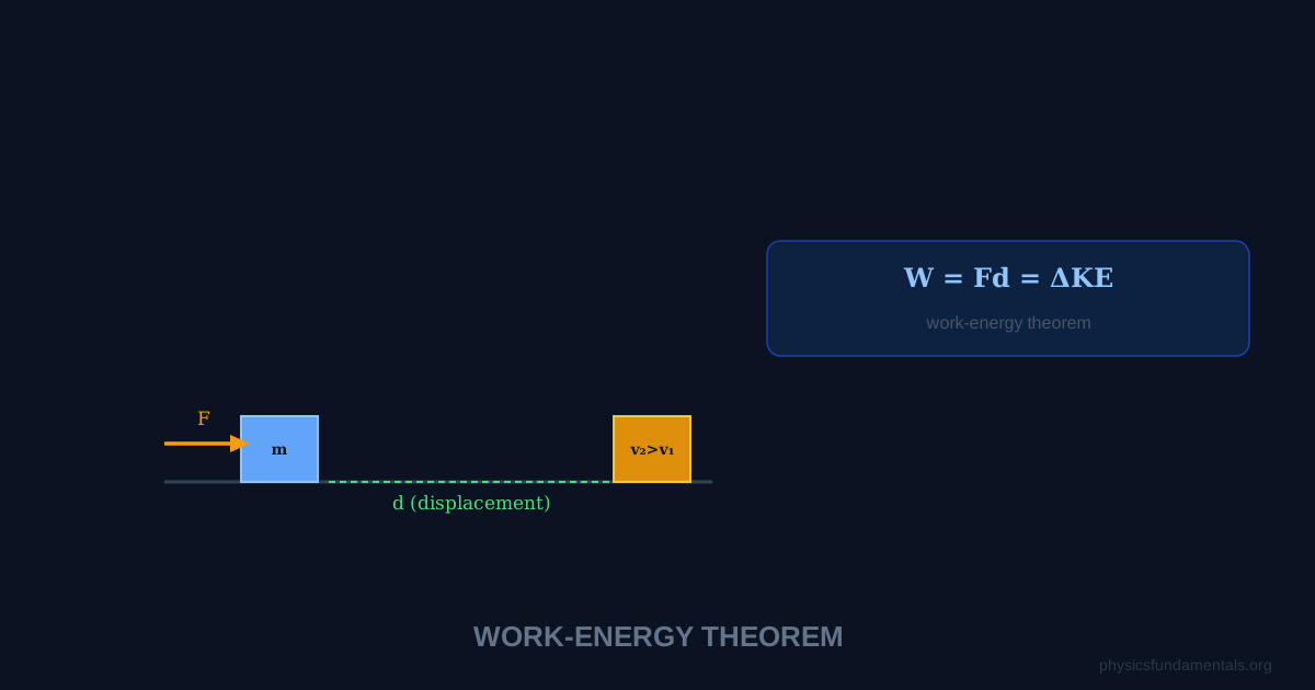
Free Fall and the Work-Energy Theorem
Free fall can also be analysed using energy conservation. A mass m falling height h in free fall gains kinetic energy equal to the loss in gravitational potential energy:
This is identical to the SUVAT result v² = 2gs (with s = h). The energy approach is often faster for problems asking for impact speed when height is given — you don't need time at all.
With air resistance present, some energy is dissipated as heat by drag. The energy equation becomes:
where W_drag is the work done against drag (always positive, always reducing final KE). This is why a real falling object hits the ground slower than a free-fall calculation predicts — some GPE went into heat rather than KE.
Free Fall in Space
Astronauts in the International Space Station (ISS) experience weightlessness not because there's no gravity — the ISS orbits at ~400 km altitude where g ≈ 8.7 m/s², still about 89% of surface gravity. They feel weightless because they are in continuous free fall around Earth. The station and everything inside it fall together at the same rate, so no contact forces act between them. This is called microgravity — there's gravity, but everything is falling together so nothing feels it.
This is exactly the equivalence principle at work: in a freely falling reference frame, gravity is locally undetectable. Einstein used this idea as the cornerstone of general relativity — the starting point being that a person in free fall has no local experiment that can distinguish between being in free fall in a gravitational field and floating in empty space far from any mass.
Frequently Asked Questions
What is free fall in physics?
What is terminal velocity?
Why do all objects fall at the same rate in a vacuum?
What factors affect terminal velocity?
What is the acceleration due to gravity g?
How do you calculate free fall velocity?
Share this article
Written by
Physics Fundamentals Editorial Team
Written and reviewed by our team of physics educators. Content is aligned with A-Level, GCSE, AP Physics, and undergraduate curricula.
About Physics Fundamentals →