Half-Life: Formula, Calculations & Worked Examples Explained

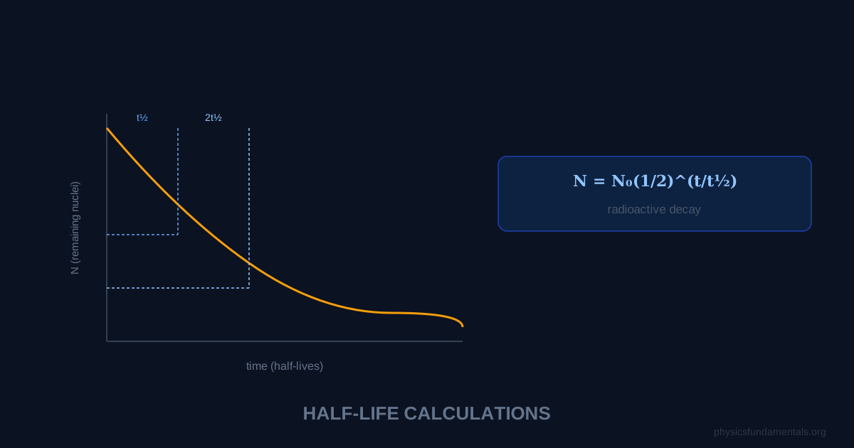
The half-life of a radioactive isotope is the time taken for half the nuclei in a sample to decay. After one half-life, half remain. After two half-lives, one quarter remain. After n half-lives, the fraction remaining is (½)ⁿ. The formula is N = N₀(½)^(t/t½), or equivalently N = N₀e^(−λt), where λ is the decay constant related to the half-life by t½ = ln2/λ ≈ 0.693/λ.

Half-life is fundamental to nuclear physics and has remarkable practical importance: it's the basis of carbon-14 dating (which can date organic material up to ~50,000 years old), the design of nuclear reactors, radiation safety planning, and medical imaging with radioisotopes. The concept is also a beautiful example of exponential decay — the same mathematical behaviour seen in capacitor discharge, cooling, and population biology.

What Is Half-Life?

The independence from sample size is crucial and non-obvious. Whether you have 1 gram or 1 tonne of carbon-14, half of it decays in 5,730 years. The decay is a purely nuclear process — it depends only on the probability that a given nucleus will decay per unit time, not on anything external to the nucleus.

The Decay Formulas

Formula 1 — Using half-lives directly

Where N is the number of nuclei remaining after time t, N₀ is the initial number, and t½ is the half-life. Use this when the time is given as a whole number of half-lives, or when you want a quick calculation.

Formula 2 — Exponential decay

Where λ is the decay constant — the probability of a given nucleus decaying per unit time (units: s⁻¹, min⁻¹, or yr⁻¹ depending on context).

Relationship between λ and t½

Both formulas give the same N for the same t — they're equivalent forms. Formula 1 is easier for whole-number multiples of t½; Formula 2 is essential for non-integer multiples.

Activity

Activity (A) is the number of decays per second — the rate at which the sample is emitting radiation:

Activity is measured in becquerels (Bq), where 1 Bq = 1 decay per second. Since N decreases exponentially, activity also decreases exponentially:

Half-Lives of Common Isotopes

Isotope	Half-life	Application
Carbon-14	5,730 years	Archaeological dating
Iodine-131	8.02 days	Medical thyroid treatment
Technetium-99m	6.01 hours	Medical imaging
Uranium-238	4.47 billion years	Geological dating, reactor fuel
Radon-222	3.82 days	Radon gas in homes
Plutonium-239	24,100 years	Nuclear weapons, reactor fuel

4 Worked Examples

Example 1 — Fraction remaining after whole half-lives

Problem: A sample of iodine-131 (t½ = 8 days) starts with 800 mg. How much remains after 32 days?

Solution:
Number of half-lives = 32/8 = 4
N = N₀ × (½)⁴ = 800 × 1/16 = 50 mg

Example 2 — Exponential decay (non-integer half-lives)

Problem: A radioactive isotope has a half-life of 12 hours. What fraction of the original sample remains after 30 hours?

Solution:
λ = ln2/t½ = 0.693/12 = 0.05776 hr⁻¹
N/N₀ = e^(−λt) = e^(−0.05776 × 30) = e^(−1.7329) = 0.177 (17.7%)
Or: N/N₀ = (½)^(30/12) = (½)^2.5 = 1/5.657 = 0.177 ✓

Example 3 — Finding the half-life from data

Problem: A sample has activity 4800 Bq at t = 0 and 300 Bq at t = 40 minutes. Find the half-life.

Solution:
A/A₀ = 300/4800 = 1/16 = (½)ⁿ → n = 4 half-lives
t½ = t/n = 40/4 = 10 minutes

Example 4 — Carbon dating

Problem: An ancient piece of wood has a carbon-14 activity of 25% of living wood activity. Estimate the age of the wood. (t½ for C-14 = 5730 years)

Solution:
A/A₀ = 0.25 = (½)^(t/5730)
0.25 = (½)² so t/5730 = 2
t = 2 × 5730 = 11,460 years

Why Does Half-Life Follow an Exponential Decay?

Each nucleus decays independently with a fixed probability λ per unit time. For a large number N of nuclei, the rate of decay is:

This differential equation has the solution N = N₀e^(−λt) — exponential decay. The key property of exponential decay is that the fraction decaying per unit time is constant (λ), even though the absolute number decaying decreases as the sample shrinks. This is why half-life is constant regardless of sample size.

Decay Constant and Its Physical Meaning

The decay constant λ (lambda) gives the probability per unit time that a single nucleus will decay. It is related to half-life by:

A large λ means rapid decay (short half-life); small λ means slow decay. The SI unit is s⁻¹ (per second). Uranium-238 has λ = 4.88 × 10⁻¹⁸ s⁻¹ — any individual nucleus has less than a 1 in 10¹⁷ chance of decaying in any given second. Carbon-14 has λ = 3.83 × 10⁻¹² s⁻¹ — still very slow, but 10⁶ times faster than U-238. Radon-222 has λ = 2.10 × 10⁻⁶ s⁻¹ and decays perceptibly within days.

Activity — Decays Per Second

Activity A is the number of decays per second (unit: becquerel, Bq = 1 decay/s):

Activity also halves every half-life. The old unit curie (Ci) = 3.7 × 10¹⁰ Bq (activity of 1 g of radium-226). A typical smoke detector contains about 37 kBq of americium-241. A PET scan uses ~400 MBq of fluorine-18. After 10 half-lives, activity has fallen to (½)¹⁰ = 1/1024 ≈ 0.1% of the original — the practical rule for "safe" decay.

Radiocarbon Dating

Carbon-14 (t½ = 5,730 years) is produced continuously in the upper atmosphere by cosmic ray neutrons striking nitrogen-14: ¹⁴N + n → ¹⁴C + p. Living organisms maintain a constant ratio of ¹⁴C/¹²C ≈ 1.3 × 10⁻¹² by continuously exchanging carbon with the atmosphere through eating and breathing. When an organism dies, it stops exchanging carbon and its ¹⁴C begins to decay. Measuring the current ¹⁴C/¹²C ratio gives the time since death:

Practical range: 300–50,000 years. Older samples have too little ¹⁴C to measure reliably. Calibration curves (from tree rings, corals, and lake sediments) correct for natural variations in atmospheric ¹⁴C concentration over time. Radiocarbon dating has revolutionised archaeology, fixing dates for events from the Turin Shroud (1260–1390 CE) to Ötzi the Iceman (3,300 BCE).

Worked Example 5 — Carbon dating a sample

Problem: An ancient wood sample has ¹⁴C activity 3.1 Bq per gram of carbon. Fresh wood has activity 14.0 Bq/g. Find the age of the sample. (t½ for ¹⁴C = 5,730 years)

Solution:
A = A₀e^{−λt} → A/A₀ = e^{−λt}
t = −(1/λ)ln(A/A₀) = (t½/ln2)ln(A₀/A)
t = (5730/0.693) × ln(14.0/3.1) = 8267 × ln(4.516) = 8267 × 1.507 = 12,460 years

Nuclear Waste and Long Half-Lives

Nuclear power produces waste containing isotopes with a huge range of half-lives. Short-lived fission products (iodine-131, t½ = 8 days; caesium-137, t½ = 30 years) are highly active initially but decay to safe levels within decades to centuries. Long-lived actinides (plutonium-239, t½ = 24,110 years; americium-241, t½ = 432 years) remain hazardous for thousands of years. Deep geological disposal in stable rock formations is the internationally agreed solution — keeping the waste isolated for the hundreds of thousands of years until radioactivity falls to background levels. The challenge is communicating the hazard across timescales longer than human civilisation has existed.

Worked Example 6 — Activity after multiple half-lives

Problem: A sample of iodine-131 (t½ = 8 days) has initial activity 6.4 × 10⁸ Bq. Find the activity after (a) 24 days, (b) 40 days.

Solution:
(a) 24 days = 3 half-lives: A = A₀ × (½)³ = 6.4 × 10⁸/8 = 8.0 × 10⁷ Bq
(b) 40 days = 5 half-lives: A = A₀ × (½)⁵ = 6.4 × 10⁸/32 = 2.0 × 10⁷ Bq

Medical Applications of Radioactive Tracers

Radioisotopes used in medicine must have half-lives long enough to allow imaging but short enough to minimise radiation dose. Technetium-99m (t½ = 6 hours) is the most widely used medical radioisotope — it emits gamma rays detectable by a gamma camera and decays to stable technetium-99 within days. PET (Positron Emission Tomography) uses fluorine-18 (t½ = 110 minutes) attached to glucose molecules: tumours and active brain regions metabolise glucose more rapidly, accumulating the tracer and emitting detectable gamma ray pairs from positron-electron annihilation. The short half-life means patients receive minimal long-term radiation dose, but it also means the isotope must be produced in a cyclotron adjacent to the hospital and used within hours.

Exponential Decay in Other Contexts

The mathematics of radioactive decay — N = N₀e^{−λt} — applies to any process where the rate of decrease is proportional to the current quantity. Exactly the same equation describes: capacitor discharge (Q = Q₀e^{−t/RC}), Newton's law of cooling (ΔT = ΔT₀e^{−kt}), pharmacokinetics (drug concentration in blood), and the attenuation of X-rays through material (I = I₀e^{−μx}). Understanding radioactive decay deeply prepares you to recognise and solve all of these exponential decay problems — they are mathematically identical, differing only in what N, λ, and t represent physically.

Exam Tips for Half-Life Problems

For a whole number of half-lives: use N = N₀ × (½)ⁿ directly, where n = t/t½. This is faster than the exponential formula and avoids logarithm errors. For non-integer numbers of half-lives: use N = N₀e^{−λt} with λ = ln2/t½, or equivalently N = N₀ × (½)^{t/t½}. Always check units: if t is in years, t½ must be in years. Common mistake: confusing activity (decays per second) with number of nuclei — they are related by A = λN, so if activity halves in one half-life and number of nuclei also halves in one half-life, both quantities follow the same exponential decay.

Worked Example 7 — Finding half-life from data

Problem: A detector records the following count rates from a pure radioactive source: 800 Bq at t = 0, 566 Bq at t = 10 min, 400 Bq at t = 20 min, 283 Bq at t = 30 min. Determine the half-life.

Solution:
Method 1 — spot the halving: count rate drops from 800 to 400 between t = 0 and t = 20 min. Therefore t½ = 20 minutes. Check: 800 → 566 ≈ 800/√2 in 10 min (one half-life = 20 min, so 10 min is half a half-life, giving factor 1/√2 ≈ 0.707, and 800 × 0.707 = 565 ✓).
Method 2 — using ln: A = A₀e^{−λt} → ln(A) = ln(A₀) − λt. Plot ln(A) vs t; gradient = −λ. From t=0 to t=20: λ = ln(800/400)/20 = ln(2)/20 = 0.0347 min⁻¹ → t½ = ln2/λ = 0.693/0.0347 = 20 min ✓

In a real experiment, always plot ln(activity) vs time — a straight line confirms pure exponential decay (single isotope), while a curve indicates multiple isotopes with different half-lives. The gradient gives λ directly.

Summary of Key Relationships

Four equivalent ways to express the decay law: N = N₀e^{−λt}; N = N₀(½)^{t/t½}; A = A₀e^{−λt}; A = A₀(½)^{t/t½}. The decay constant λ = ln2/t½ = 0.693/t½ converts between these forms. The mean lifetime τ = 1/λ = t½/ln2 = 1.443 × t½ is the average time a nucleus survives before decaying (slightly longer than t½ because the distribution is exponential, not uniform). In time τ, the activity falls to 1/e ≈ 36.8% of its initial value. Both t½ and τ appear in physics problems — know which is which.

Background Radiation and Corrected Count Rates

Every radiation detector measures background radiation in addition to the source — cosmic rays, natural radioactive materials in buildings, and trace radioactive isotopes in soil. Before using any count rate in decay calculations, subtract the background: A_corrected = A_measured − A_background. A typical laboratory background count rate is 20–50 counts per minute. For a source initially giving 2000 counts/min, the background correction is small (1–2%). For a source that has decayed to 60 counts/min, background of 40 cpm becomes a 67% correction — dominant. Always measure background before and after the experiment and use the average. Ignoring background is the most common systematic error in school half-life experiments using short-lived sources like protactinium-234 (t½ = 70 s).

Half-life problems are among the most numerically reliable in A-Level physics — the decay law is exact (not an approximation), the formula is clean, and errors are usually from incorrect unit conversions or forgetting to subtract background. Three worked strategies: (1) count the number of half-lives and use (½)ⁿ — fastest for integer half-lives; (2) use N = N₀e^{−λt} with λ = ln2/t½ — best for non-integer times; (3) take natural logs of N = N₀e^{−λt} to get ln(N) = ln(N₀) − λt — rearrange for any unknown. For graphical analysis, always plot ln(N) or ln(A) vs time — the resulting straight line has gradient −λ and y-intercept ln(N₀), from which both λ and t½ are extractable with high accuracy.